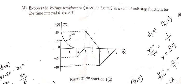
I am confused with how to put e^(-2t) in terms of u(t). Also please what will be the entire equation. Thank you in advance.
please could you solve these questions for me?
When acquiring experimental data, the analog signal is digitized through an A/D converter.
Consequentially, all of the values calculated or derived from those data are only estimations of
the true values (recall that DAQ devices have quantization errors). Consider an analog signal
that is a sine wave with a frequency of f = 2 Hz, an amplitude A = 1.5, and a phase lag
that is equivalent to τ = 0.8 seconds. Let’s call this analog signal x(t).
(a) Determine the autocorrelation for x(t) analytically (i.e., evaluate the following equation
for some value “t0” by hand)
Rxx(t0,τ) = E[x(t0)x(t0+ τ)]
(b) What effect does t0have on the autocorrelation? What are the implications of this?
(c) Discretize x(t) using a sampling frequency of fs= 100 Hz for 0 ≤ t ≤ 2 s. This will
simulate you having acquired the data with no quantization errors.
(d) Using the discretized signal, compute the autocorrelation of x(n∆t) using both the ‘biased’
and ‘unbiased’ scaling options for the xcorr() command in MATLAB.
(e) Plot all three autocorrelations (your analytical solution, the biased output, and the unbi-
ased output) on the same figure (one single axis), showing only the results for 0 ≤lags ≤
200 [points].
Note: You also have to discretize the analytical solution from part (a). You can convert
between τ and lags using the following equation: τ = lags/fs.
(f) Explain your results. Why is there a difference between the three plots?
- Write a script to calculate both the power spectrum and power spectral density of a signal
using the formulas from the lecture notes. Do not use the pwelch(), cpsd(), or spectrogram()
commands in your script. Use a single block of data (i.e., no overlap) and a rectangular
window for this analysis.
(a) Plot the results (power spectrum and power spectral density) for the following signal with
an integer number of periods in the record length you choose, T.
x(t) = 2.3 sin (2π150t) + 0.9 sin (2π60t) + 1.7
(b) What values did you choose for fs, T, N, and ∆f? Before proceeding, if you have ∆f = 1
Hz, change your values so ∆f 6= 1 Hz and list out your new values.
(c) Tabulate the quantities of the computed power spectrum and power spectral density at
DC, at 60 Hz, and at 150 Hz.
(d) Verify that Parseval’s theorem holds. Adjust the mean value and amplitudes of the terms
to verify that your code works properly.
(e) Verify the PSD of the signal in part (a) by producing an additional plot using the pwelch()
command. (Make a new plot comparing your power spectral density and that of the
pwelch() output
